Inference
This document partially covers the following modules:
tramway.analyzer.mappertramway.analyzer.browser
![]()
Like most of the pages of this documentation, this one originates from a IPython notebook and, as a consequence, the code examples are sequentially run, hence the inclusion of a few transition steps.
TRamWAy features multiple models to infer physical properties of random walks, including diffusivity, effective potential, drift, force, etc. Most of the available models are based on the overdamped Langevin equation.
Models for random walks
For extensive introduction, please refer to the official documentation and the InferenceMAP paper and webpage.
Briefly, we consider the problem of maximizing the posterior probability for model parameters \(\theta\) given the observed particle displacements \(T_i = {(\Delta t_j, \Delta\textbf{r}_j)}\) partitioned into bins or microdomains whose index is denoted by \(i\):
The various models TRamWAy features give different formulae for the local likelihoods \(P(T_i|\theta_i)\). In addition, \(P(\theta)\) can be treated as a regularization term, often in the shape of an improper prior (not normalized).
The main models are recaped in the following table:
| model name | model parameters | equation for the individual displacements |
|---|---|---|
| D 1 2 | diffusivity \(D\) | \(\frac{d\textbf{r}}{dt} = \sqrt{2D(\textbf{r})} \xi(t)\) |
| DD 1 2 | diffusivity \(D\) drift \(\textbf{a}\) |
\(\frac{d\textbf{r}}{dt} = \sqrt{2D(\textbf{r})} \xi(t) + \textbf{a}(\textbf{r})\) |
| DF 1 2 | diffusivity \(D\) force \(\textbf{F}\) |
\(\frac{d\textbf{r}}{dt} = \sqrt{2D(\textbf{r})} \xi(t) + D(\textbf{r})\frac{\textbf{F}(\textbf{r})}{k_{\textrm{B}}T}\) |
| DV 1 2 | diffusivity \(D\) effective potential \(V\) |
\(\frac{d\textbf{r}}{dt} = \sqrt{2D(\textbf{r})} \xi(t) - D(\textbf{r}) \frac{\nabla V(\textbf{r})}{k_{\textrm{B}}T}\) |
The stochastic variant for the DV model is covered in more details.
from tramway.analyzer import *
import numpy as np
from src.inference import set_notebook_theme
# this actually does something only for *dark* themes
set_notebook_theme('light')
from matplotlib import pyplot as plt
The preset analyzer is programmed to load a designated SPT data file, extract the data in a single region of interest, build a k-means-based tessellation, and assign the particle locations to the different Voronoi cells with an additional adjustment to ensure at least 10 locations are associated with each cell.
from src.inference import reset_data, preset_analyzer
reset_data()
Localization error
All the models above derive a similar likelihood function. As an example, for the DV model, at bin \(i\) with assigned displacements \(T_i\), the local likelihood is:
with \(\sigma^2\) the experimental localization error.
Because \(\sigma\) is a parameter of the experimental setup and protocol, it can be set and found in the spt_data attribute:
a, _ = preset_analyzer()
a.spt_data.localization_precision
0.02
localization_precision is actually a property that sets/reflects the localization_error attribute, which corresponds to \(\sigma^2\):
a.spt_data.localization_error
0.0004
Such a piece of information is required at several stages of a typical processing chain.
For convenience, the localization_precision and localization_error attributes are also exposed by the RWAnalyzer object and the mapper attribute, and point to the same value in memory, with the localization_precision properties returning the square-root of localization_error.
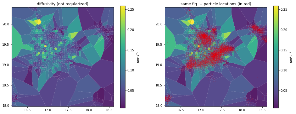
D
Assuming the dynamics is solely diffusive in nature, the following likelihood is considered at bin \(i\), with observed displacements \(T_i\):
with \(\sigma^2\) the localization error.
d_analyzer, assignment = preset_analyzer()
d_analyzer.mapper = mapper.MapperPlugin('d')
%%time
d_map = d_analyzer.mapper.infer(assignment)
CPU times: user 2.46 s, sys: 81.6 ms, total: 2.55 s
Wall time: 2.48 s
See the Data structures section for more information about the returned object.
_, axes = plt.subplots(1, 2, figsize=(16,6))
d_analyzer.mapper.mpl.plot(d_map, 'diffusivity', assignment, axes=axes[0], title='diffusivity (not regularized)', unit='std')
d_analyzer.mapper.mpl.plot(d_map, 'diffusivity', assignment, axes=axes[1], title='same fig. + particle locations (in red)', unit='std', overlay_locations=True)
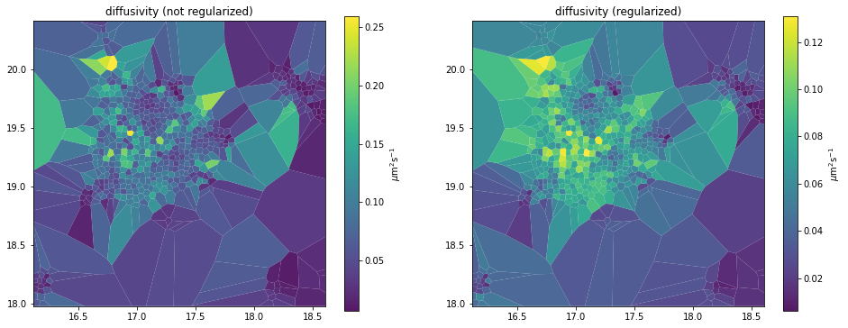
Smoothing regularizers
To properly estimate the local diffusivity with few data points, we make use of regularizing priors that smooth the diffusivity landscape.
The 'd', 'dd', 'df' and 'dv' models feature the following default penalty on the diffusivity \(D\):
with \(\mathcal{A}_i\) the surface area (or volume) of bin \(i\), and \((\nabla D)_i\) the gradient of \(D\) at bin \(i\).
reg_d_analyzer, assignment = preset_analyzer()
reg_d_analyzer.mapper = mapper.MapperPlugin('d')
The \(\lambda\) hyperparameter can be set as follows:
m = assignment.number_of_cells # number of bins
n = len(assignment) # number of assigned translocations
roi_surface_area = 2.5 * 2.5 # in µm²
# how large can be a difference in values over a 1-µm distance?
expected_high_delta_D = .3 # in µm²s⁻¹
diffusivity_prior_z = expected_high_delta_D ** 2 * roi_surface_area * m
reg_d_analyzer.mapper.diffusivity_prior = (30 * n) / diffusivity_prior_z
Although the above value of 30 is still to be adjusted, e.g. depending on the size of the expected pattern in the diffusivity landscape, the proposed normalization makes this value less variable from a dataset to another.
Indeed, the log-likelihood term in the cost function is a sum over all translocations (n), while the regularizing term is a sum over all bins (m).
Be careful however, when exploring the hyperparameter space, that it may take much more time for the inference to converge at higher weights on the regularizing prior. If this happens, as long as at least one iteration was performed, you can interrupt the interpreter with Ctrl+C, or the Interrupt the kernel button in a notebook. The solution at the last iteration is returned and the program execution proceeds.
In addition to this smoothing prior, we can also prevent the estimated diffusivity values to become negative, using a Jeffreys' prior:
reg_d_analyzer.mapper.jeffreys_prior = True
A better way to prevent the diffusivity to take negative values would consist of removing the static trajectories. Such a preprocessing step is skipped here, but systematically performed by the building blocks mentioned further.
Here, we stick to the Jeffreys' prior solution for comparing with the regularization-free approach.
%%time
reg_d_map = reg_d_analyzer.mapper.infer(assignment)
CPU times: user 8h 10min 58s, sys: 47.5 s, total: 8h 11min 46s
Wall time: 8h 10min 42s
See the Data structures section for more information about the returned object.
_, axes = plt.subplots(1, 2, figsize=(16,6))
d_analyzer.mapper.mpl.plot(d_map, 'diffusivity', assignment, axes=axes[0], title='diffusivity (not regularized)', unit='std')
reg_d_analyzer.mapper.mpl.plot(reg_d_map, 'diffusivity', assignment, axes=axes[1], title='diffusivity (regularized)', unit='std')
See also the Spatial smoothing priors section of the original documentation.
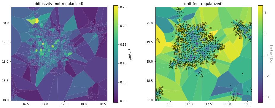
DD
This model estimates the local drift \(\textbf{a}(\textbf{r})\) in a straight-forward fashion, with the following likelihood at bin \(i\) and observed displacements \(T_i\):
with \(\sigma^2\) the localization error.
dd_analyzer, assignment = preset_analyzer()
dd_analyzer.mapper = mapper.MapperPlugin('dd')
The mapper attribute for 'dd' features the diffusivity_prior and drift_prior smoothing hyperparameters.
%%time
dd_maps = dd_analyzer.mapper.infer(assignment)
CPU times: user 3.81 s, sys: 15 µs, total: 3.81 s
Wall time: 3.79 s
See the Data structures section for more information about the returned object.
_, axes = plt.subplots(1, 2, figsize=(16,6))
dd_analyzer.mapper.mpl.plot(dd_maps, 'diffusivity', assignment, axes=axes[0], title='diffusivity (not regularized)', unit='std')
dd_analyzer.mapper.mpl.plot(dd_maps, 'drift', assignment, axes=axes[1], title='drift (not regularized)', unit='log[ µm / s ]', transform='log')
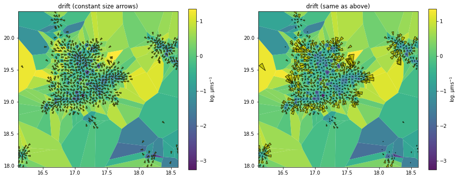
Arrow scaling in field maps
_, axes = plt.subplots(1, 2, figsize=(16,6))
common_args = (dd_maps, 'drift', assignment)
common_kwargs = dict(unit='std', transform='log')
dd_analyzer.mapper.mpl.plot(*common_args, **common_kwargs,
axes=axes[0], title='drift (constant size arrows)',
arrow_size='constant', cell_arrow_ratio=1.3) # cell_arrow_ratio is optional
dd_analyzer.mapper.mpl.plot(*common_args, **common_kwargs,
axes=axes[1], title='drift (same as above)')
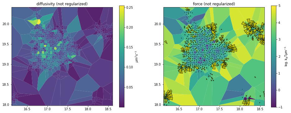
DF
Building upon the DD model, the drift is explained by a force \(\textbf{F}\) and friction \(\gamma\): \(\textbf{a}(\textbf{r}) = \frac{\textbf{F}(\textbf{r})}{\gamma(\textbf{r})}\). In addition, assuming equilibrium: \(\gamma(\textbf{r}) = \frac{k_{\textrm{B}}T}{D(\textbf{r})}\).
As a consequence, the following likelihood is considered at bin \(i\), with observed displacements \(T_i\):
with \(\sigma^2\) the localization error.
df_analyzer, assignment = preset_analyzer()
df_analyzer.mapper = mapper.MapperPlugin('df')
The mapper attribute for 'df' features the diffusivity_prior and force_prior smoothing hyperparameters.
%%time
df_maps = df_analyzer.mapper.infer(assignment)
CPU times: user 6.26 s, sys: 124 ms, total: 6.38 s
Wall time: 6.24 s
See the Data structures section for more information about the returned object.
_, axes = plt.subplots(1, 2, figsize=(16,6))
df_analyzer.mapper.mpl.plot(df_maps, 'diffusivity', assignment, axes=axes[0], title='diffusivity (not regularized)', unit='std')
df_analyzer.mapper.mpl.plot(df_maps, 'force', assignment, axes=axes[1], title='force (not regularized)', clim=[-1,5], clip=3, unit='std', transform='log')
DV
Building upon the DF model, the force field is assumed to be conservative and result from a potential energy: \(\textbf{F}(\textbf{r}) = -\nabla V(\textbf{r})\).
The following likelihood is considered at bin \(i\), with observed displacements \(T_i\):
with \(\sigma^2\) the localization error. In practice, TRamWAy estimates the dimension-less ratio \(\frac{V}{k_{\textrm{B}}T}\) and \(V\) is expressed as multiples of \(k_{\textrm{B}}T\).
dv_analyzer, assignment = preset_analyzer()
dv_analyzer.mapper = models.DV()
mapper.MapperPlugin('dv') is also available but its naive implementation makes it far too slow for the example 635-bin segmentation.
We recommend using models.DV() instead which wraps an alternative implementation with a faster gradient calculation for the cost function to be minimized.
Note however that models.DV() also features an alternative regularizer.
The mapper attribute for mapper.MapperPlugin('dv') and models.DV() features the diffusivity_prior and potential_prior smoothing hyperparameters.
The effective potential is implicitly smoothed, already, due to the calculation of \(\nabla V\). The DV model is slow for the same reason, that also requires all the parameters to be jointly optimized.
Stochastic DV
A faster stochastic implementation of the DV model is available in two flavors: either fully stochastic ('stochastic.dv' plugin or models.DV(variant='stochastic')), or two-phase with the stochastic approach used first and the standard approach used second for fine-tuning ('semi.stochastic.dv' plugin or models.DV(start='stochastic')).
The stochastic method is described in a published article. As observed in that work, the stochastic variant works well to reach a basin around the solution, and then underperforms within the basin. That is why we recommend the semi-stochastic approach with a predetermined number of stochastic steps followed by non-stochastic fine-tuning.
Among other benefits of reducing the complexity of the inference, this method makes spatio-temporal inferences possible, that regularize the dynamics parameters across time.
sdv_analyzer, assignment = preset_analyzer()
sdv_analyzer.mapper = models.DV(start='stochastic')
Setting the smoothing priors
The 'stochastic.dv' model features an alternative penalty on the diffusivity \(D\) (and similarly on the effective potential \(V\)):
with \(i\) all the existing bin/microdomain indices and \(N_i\) the subset of neighbor bins.
This is used as a prior probability function but, just like the default smoothing prior for the other algorithms, is not a proper probability function. Per default, no normalization is performed to allow maximum control on the regularization effect, especially across multiple datasets.
Here we normalize as follows:
m = assignment.number_of_cells # number of bins
n = len(assignment) # number of assigned translocations
roi_surface_area = 2.5 * 2.5 # in µm²
# how large can be a difference in values over a 1-µm distance?
expected_high_delta_D = .3 # in µm² s⁻¹
expected_high_delta_V = 5 # in kT
diffusivity_prior_z = expected_high_delta_D ** 2 * roi_surface_area * m
potential_prior_z = expected_high_delta_V ** 2 * roi_surface_area * m
Due to \(\nabla V\) already smoothing the landscape of \(V\), we can penalize the spatial variations of \(V\) to a lesser extent than those of \(D\).
Compared with the original smoothing prior from InferenceMAP, we will consider lower weights for this prior, usually 4 times lower to account for how \(\nabla V\) is calculated and how many times each difference is counted and scaled.
Again, higher weights on the diffusivity smoothing prior usually make the inference take quite a lot more time, but in the case the inference takes too long, you can interrupt it with Ctrl+C, or the Interrupt the kernel square button in a notebook.
sdv_analyzer.mapper.diffusivity_prior = (7.5 * n) / diffusivity_prior_z
sdv_analyzer.mapper.potential_prior = (0.5 * n) / potential_prior_z
((7.5 * n) / diffusivity_prior_z, (0.5 * n) / potential_prior_z)
(259.2755905511811, 0.06222614173228346)
Running the inference
This is done calling the infer method, passing as input argument the assignment previously given by the sample method.
%%time
sdv_maps = sdv_analyzer.mapper.infer(assignment)
CPU times: user 3min 24s, sys: 9.39 s, total: 3min 33s
Wall time: 9min 5s
See the Data structures section for more information about the returned object.
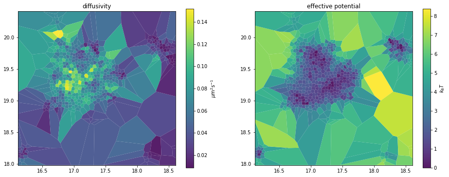
Plotting the inferred parameters
_, axes = plt.subplots(1, 2, figsize=(16,6))
sdv_analyzer.mapper.mpl.plot(sdv_maps, 'diffusivity', assignment, axes=axes[0], title='diffusivity', unit='std')
sdv_analyzer.mapper.mpl.plot(sdv_maps, 'potential', assignment, axes=axes[1], title='effective potential', unit='std')
Saving parameter maps to .rwa files
In the above example, with a single set of maps on a single region of interest, we can explicitly dump the above assignment and maps in a .rwa file:
import os.path
a = sdv_analyzer # any of the previously-defined analyzer accesses the same file and can be used here
rwa_file = os.path.splitext(a.spt_data.filepath)[0] + '.rwa'
with a.spt_data.autosaving() as analysis_tree:
analysis_tree.rwa_file = rwa_file
analysis_tree['my roi'] = assignment
analysis_tree['my roi']['my maps 0'] = reg_d_map
analysis_tree['my roi']['my maps 1'] = sdv_maps
This appends the new records to the existing analyses if the file already exists.
The structure of an analysis tree is flexible, but preferably includes the full SPT data at the root node (as a DataFrame object), the different assignments as immediate children nodes (as Partition objects), and finally the inferred maps as grand-children (as Maps objects):
print(analysis_tree)
<class 'pandas.core.frame.DataFrame'>
'my roi' <class 'tramway.tessellation.base.Partition'>
'my maps 0' <class 'tramway.inference.base.Maps'>
'my maps 1' <class 'tramway.inference.base.Maps'>
This analysis tree can be loaded using the load_rwa function exported by the tramway.helper module:
%%script echo skipping
from tramway.helper import load_rwa
reloaded_analysis_tree = load_rwa(rwa_file)
print(reloaded_analysis_tree)
assignment = reloaded_analysis_tree['my roi'].data
reg_d_map = reloaded_analysis_tree['my roi']['my maps 0'].data
skipping
Generally speaking, inspecting a .rwa file may be easier without the help of the RWAnalyzer object, and the reader is referred to the command-line interface or the tramway.helper package for functions like load_rwa, cell_plot or map_plot.
Indeed, an RWAnalyzer object cannot be loaded directly from a .rwa file.
Especially, a single RWAnalyzer object may handle multiple files, and a .rwa file may contain analysis artefacts generated by different RWAnalyzer objects.
In addition, even a specific analysis path from a .rwa file does not contain enough information to rebuild an RWAnalyzer object.
First, we would need to have the region of interest defined in an additional file. Such a file can be generated as follows:
roi_file = os.path.splitext(a.spt_data.filepath)[0] + '-roi.txt'
f = single(a.spt_data)
f.roi.to_ascii_file(roi_file)
See the roi notebook/section about ROI for more information.
However, an analysis based on a RWAnalyzer object is mostly declarative. The entire computation can be described as a series of attribute assignments, and eventually triggered by a single line of code.
Segmenting and inferring all at once
To further ease the manipulation of data files, including .rwa files, the tramway.analyzer package features some convenient building blocks, especially tessellate_and_infer.
For example, to reproduce the steps of the DV inference above, on top of a k-means-based tessellation with local adjustments to reach a minimum number of 10 data points per space bin:
from tramway.analyzer import *
import numpy as np
import pandas as pd
a = RWAnalyzer()
a.spt_data.from_ascii_file('../data/Image_traj.txt')
a.spt_data.frame_interval = .04 # in s
a.spt_data.localization_precision = .02 # in µm
a.roi.from_ascii_files() # default filepath will be '../data/Image_traj-roi.txt'
a.tesseller = tessellers.KMeans
a.tesseller.resolution = .05 # in µm
a.sampler = sampler.Knn(10)
a.mapper = models.DV(start='stochastic')
# details about the hyperparameters below are omitted
a.mapper.diffusivity_prior = 259.27
a.mapper.potential_prior = 0.062226
a.pipeline.append_stage(stages.tessellate_and_infer(sampling_label='my roi', map_label='my map 0'))
The last expression above does not run the computation. It only schedules it for later execution by the run method. The resulting analysis artefacts are saved in a .rwa file whose name per default is borrowed by the SPT data filename, replacing the original extension by the .rwa extension.
Note that tessellate_and_infer (similarly tessellate) will discard the static trajectories.
This additional preprocessing step was not performed by the preset_analyzer function to keep it as simple as possible.
With a few additional lines, the computation can be dispatched to a computer cluster instead of being run on the local machine. This, however, is out of the scope of this section.
The computation can be triggered calling the run method:
%%script echo skipping
a.pipeline.run()
skipping
We skip the execution of the above run call so that the present document (originally a Jupyter notebook) can be run in a limited amount of time.
Post-processing
Instead, if the .rwa file already exists, we can load and manipulate it:
stages.reload(skip_missing=False)(a)
To show the same maps as above, in a different flavor, let us plot 3D surfaces:
%%capture
import sys
!"{sys.executable}" -m pip install plotly nbformat
from plotly.io import renderers
renderers.default = 'notebook'
from plotly.subplots import make_subplots
from IPython.display import HTML, display
for r in a.roi.as_support_regions(): # in this example, we have a single ROI
assignment = r.get_sampling('my roi')
maps = assignment.get_child('my maps 1')
fig = make_subplots(rows=1, cols=2,
specs=[[{'type': 'surface'}, {'type': 'surface'}]],
subplot_titles=['diffusivity', 'effective potential'])
a.mapper.plotly.plot_surface(maps, 'diffusivity', assignment, fig=fig, col=0,
colorbar=dict(thickness=20, x=0.46))
a.mapper.plotly.plot_surface(maps, 'potential', assignment, fig=fig, col=1,
colorbar=dict(thickness=20, x=1.02))
fig.update_layout(
scene1=dict(
zaxis=dict(range=[-.08,.15]),
camera=dict(eye=dict(x=.8, y=.8, z=1.4)),
),
scene2=dict(
zaxis=dict(range=[-2,8.3]),
camera=dict(eye=dict(x=.5, y=.5, z=2.)),
),
)
# fig.show() # nbconvert cannot export the figure this way
display(HTML(fig.to_html())) # .. so we call this expression instead
Data structures
The Maps objects previously generated, for example sdv_maps, contain the distributed parameter estimates:
print(sdv_maps)
mode: semi.stochastic.dv
diffusivity_prior: 259.2755905511811
potential_prior: 0.06222614173228346
runtime: 544.6461782455444
ls_step_max: [0.025 0.5 ]
ftol: 0.001
low_df_rate: 1
allow_negative_potential: True
max_iter: 20
sigma: 0.02
verbose: False
resolution: CONVERGENCE: DELTA F <= FTOL/10
niter: 2
init: {'resolution': 'CONVERGENCE: DELTA F < FTOL', 'niter': 43387}
features: ['diffusivity', 'potential', 'force']
maps: <class 'pandas.core.frame.DataFrame'>
The values can either be accessed reading the maps attribute:
import pandas as pd
pd.set_option('display.max_rows', 6)
sdv_maps.maps
| diffusivity | potential | force x | force y | |
|---|---|---|---|---|
| 0 | 0.054227 | 4.979276 | 1.024797 | 14.472462 |
| 1 | 0.046272 | 5.025369 | 21.527693 | 14.087935 |
| 2 | 0.024227 | 2.360643 | 20.089187 | 26.576126 |
| ... | ... | ... | ... | ... |
| 632 | 0.024116 | 4.559752 | 3.570716 | 2.587393 |
| 633 | 0.030418 | 4.236661 | -16.891351 | -5.274054 |
| 634 | 0.045488 | 4.567865 | -6.523572 | -2.787153 |
635 rows × 4 columns
or indexing by parameter name, which may prove convenient for multidimensional measurements:
sdv_maps['force'].rename(columns=lambda name: name.split()[1])
| x | y | |
|---|---|---|
| 0 | 1.024797 | 14.472462 |
| 1 | 21.527693 | 14.087935 |
| 2 | 20.089187 | 26.576126 |
| ... | ... | ... |
| 632 | 3.570716 | 2.587393 |
| 633 | -16.891351 | -5.274054 |
| 634 | -6.523572 | -2.787153 |
635 rows × 2 columns
Spatiotemporal resolution of the DV model
In combination with a sliding time window, the SPT data can be segmented in time, in addition to space.
Although it is possible to perform the inference on each time segment independently, it is also possible to run a larger inference for all the dynamics parameters at once, taking benefit from temporal regularization.
This latter approach, however, is far more time-consuming and the 'stochastic.dv' or 'semi.stochastic.dv' algorithms are recommended.
To decrease the number of empty spatiotemporal bins, we will typically decrease the spatial resolution (i.e. increase the value of the resolution attribute that actually represents the bin size).
Let us first set a similar analyzer, compared with the space-only stochastic DV approach, exposing the details that were previously hidden in the preset_analyzer function:
from tramway.analyzer import *
import numpy as np
import pandas as pd
dv_t = RWAnalyzer()
dv_t.spt_data.from_ascii_file('../data/Image_traj.txt')
dv_t.spt_data.frame_interval = .04 # in s
dv_t.spt_data.localization_precision = .02 # in µm
dv_t.roi.from_ascii_files() # default filepath will be '../data/Image_traj-roi.txt'
dv_t.tesseller = tessellers.KMeans
dv_t.tesseller.resolution = .1 # in µm
dv_t.sampler = sampler.Knn(10)
dv_t.mapper = models.DV(start='stochastic')
We first specify the temporal segmentation and regularization hyperparameters:
dv_t.time = time.SlidingWindow(duration=60, shift=30)
Next, to set the spatial regularization hyperparameters, let us generate an assignment (the assignment, here, as we have a single ROI or dataset) to read the number of spatial bins and assigned translocations. The time window must be defined first:
r = single(dv_t.roi)
df = r.discard_static_trajectories(r.crop())
assignment_t = dv_t.sampler.sample(df)
spatial_mesh = dv_t.time.get_spatial_segmentation(assignment_t)
m = spatial_mesh.number_of_cells # number of bins (per time segment)
n = len(assignment_t) # number of assigned translocations
roi_surface_area = 2.5 * 2.5 # in µm²
# how large can be a difference in values over a 1-µm distance?
expected_high_delta_D = .3 # in µm² s⁻¹
expected_high_delta_V = 5 # in kT
diffusivity_prior_z = expected_high_delta_D ** 2 * roi_surface_area * m
potential_prior_z = expected_high_delta_V ** 2 * roi_surface_area * m
Because we split the SPT data in multiple time segments, the proportion of bins that overlap with their neighbors increases, which makes the inferred landscapes smoother (in each time segment) even with no regularization. As a consequence, we decrease the weights for the spatial regularization terms, compared with a time-free assignment with equal resolution.
In addition, regularizing in time is more difficult than in space, because of the very low temporal resolution of the segmentation. Here, we have a 30-s shift between successive segments. The spatial and temporal regularizations may conflict with one another, hence the extra complexity in adjusting the hyperparameters.
weight = 1e-2
dv_t.mapper.diffusivity_prior = (7.5 * weight * n) / diffusivity_prior_z
dv_t.mapper.potential_prior = (.5 * weight * n) / potential_prior_z
dv_t.mapper.diffusivity_time_prior = 100.
dv_t.mapper.potential_time_prior = 100.
Last, we run as usual:
sampling_label = lambda roi_label: roi_label + ' - kmeans + 60s window'
map_label = 'dv maps'
dv_t.pipeline.append_stage(stages.tessellate_and_infer(
sampling_label=sampling_label,
map_label=map_label,
load_rwa_files=True,
overwrite=True,
))
%%time
dv_t.pipeline.run()
loading .rwa file for source: ../data/Image_traj.txt...
tessellating roi: 'roi000' (in source '../data/Image_traj.txt')...
inferring roi: 'roi000' (in source '../data/Image_traj.txt')...
CPU times: user 19min 58s, sys: 50.2 s, total: 20min 49s
Wall time: 1h 24min 42s
sampling_label
If no ROI are defined, it is safe to pass a static str value.
If ROI are defined and a single segmentation per ROI is expected, it is safe to ignore the sampling_label argument.
However, if ROI are defined and segmenting in multiple ways is not excluded, it is recommended to choose labels that refer both to the ROI and the segmentation parameters; hence the above sampling_label that takes the default ROI label and combines it with an additional segmentation-related label.
load_rwa_files and overwrite
Per default, if the SPT data source is not defined as .rwa files, tessellate_and_infer seeks for corresponding .rwa files and loads them if found. The load_rwa_files argument controls this behavior and can be set to False to override the default.
Per default, if the SPT data source is read from .rwa files, including by the action of the load_rwa_files argument, if analysis artefacts are already available in the analysis trees with the same labels, the analysis is skipped. The overwrite argument controls this behavior and can be set to True to override the default.
Movie rendering
Dynamic maps can be rendered as movies:
r = single(dv_t.roi)
assignment_t = r.get_sampling(sampling_label)
dv_t_maps = assignment_t.get_child(map_label)
%%capture
# initialize the movie for a parameter map
from matplotlib import pyplot as plt
fig, ax = plt.subplots(figsize=(8,6))
movie = dv_t.mapper.mpl.animate(fig, dv_t_maps, feature='diffusivity',
axes=ax, unit='std', overlay_locations=True)
# render the movie
from IPython.display import HTML
HTML(movie.to_jshtml())
The movie object is a Matplotlib animation. Such objects can be combined as subplots of a same figure:
%%capture
fig, axes = plt.subplots(1, 2, figsize=(16,6))
movie = dv_t.mapper.mpl.animate(fig, dv_t_maps, feature='diffusivity',
axes=axes[0], unit='std')
movie = dv_t.mapper.mpl.animate(movie, dv_t_maps, feature='potential',
axes=axes[1], unit='std')
HTML(movie.to_jshtml())
Note that, in the second call to animate, movie is passed as first argument instead of fig.
Browsing many maps
For datasets with multiple SPT data files and/or multiple regions of interest per files, or else multiple segmentations per region of interest and/or multiple inferred parameter maps per assignment,
the RWAnalyzer object features a browsing utility based on the Bokeh library and made available as the browser attribute of the object.
%%capture
import sys
!"{sys.executable}" -m pip install "bokeh==2.2.3"
from tramway.analyzer import *
a = RWAnalyzer()
a.spt_data.from_rwa_files('../data/*.rwa')
# the notebook kernel is not aware of the notebook it runs;
# let it know where the code is
a.browser.script = 'inference.ipynb'
# make bokeh run the current notebook cell only, not the entire notebook
a.browser.this_notebook_cell_only = True
a.browser.show_maps()
the designated .ipynb file will be exported;
be sure to save the notebook after any modification
so that the changes are reported in the .ipynb file
running: jupyter nbconvert --to python "inference.ipynb" --stdout
running: python -m bokeh serve --show /tmp/tmpccmdvbt3.py
interrupt the kernel to stop bokeh and proceed back in the notebook
2021-07-17 03:18:32,405 Starting Bokeh server version 2.2.3 (running on Tornado 6.1)
2021-07-17 03:18:32,407 User authentication hooks NOT provided (default user enabled)
2021-07-17 03:18:32,414 Bokeh app running at: http://localhost:5006/tmpccmdvbt3
2021-07-17 03:18:32,415 Starting Bokeh server with process id: 1565566
2021-07-17 03:18:39,212 W-1000 (MISSING_RENDERERS): Plot has no renderers: Figure(id='1007', ...)
2021-07-17 03:18:41,103 404 GET /favicon.ico (127.0.0.1) 1.14ms
2021-07-17 03:18:41,115 WebSocket connection opened
2021-07-17 03:18:41,117 ServerConnection created
At this point the kernel is blocking and waiting for bokeh serve to be halted. In the standard Jupyter interface, you can do so pressing the Interrupt the kernel square button, or Ctrl+C.
A new window or tab should open in your default web browser. Otherwise, the web interface Bokeh serves should be available on https://localhost:5006/. Be careful that if the notebook is accessed through an SSH tunnel, so should be the bokeh web interface.
The above code calls a highly experimental feature. The notebook cell should properly run if taken out of the notebook, and therefore include all the necessary imports.
It should not include any IPython magic statements, and the expressions that set the script and this_notebook_cell_only attributes should be in the cell code, not in imported code, as well as the browser.show_maps method call.
The corresponding strings are looked up for in the cell code.
If multiple notebook cells call browser.show_maps, attribute this_notebook_cell_only should be the cell index in the notebook, in all such cells.
![]()